Linear Fit using Python and NumPy
I was working on a side project where I needed to find the linear fit to a set of data points. A linear fit is also known as a “linear approximation” or “linear regression”. This is quite easy using a Numbers spreadsheet. Numbers will even show you equation of the line in slope-intercept form:
\[y = mx + b\]Unfortunately, there is no way that I know of to get the slope and Y-intercept from the Numbers plot besides visual inspection. I also wanted a way to do this from the command line. This post will explain how to do this using Python and the NumPy library.
TLDR: Python One-Liners
While the rest of the post goes into more detail, here are two quick Python one-liners to find the slope and Y-intercept, given two NumPy arrays, x and y. First, with Polynomial.fit():
b, m = np.polynomial.polynomial.Polynomial.fit(x, y, 1).convert().coef
And second, with Polynomial.polyfit():
b, m = np.polynomial.polynomial.polyfit(x, y, 1)
Both of these give you the slope in m and the Y-intercept in b. I also created a Jupyter notebook demonstrating these APIs.
I’m honestly not sure why you would pick one over the other. Polynomial.polyfit() is less code, so that seems like the better option, to me. But if you know, please contact me! And please read on for more details.
Using Numbers
Here’s the sample data we’ll be using throughout the rest of the post:
| X | Y |
|---|---|
| 0 | -1 |
| 1 | 0.2 |
| 2 | 0.9 |
| 3 | 2.1 |
In Numbers, put this X and Y data into a table. Then add a Scatter Plot and enable a “Linear Trendline” with “Show Equation” checked. You should see a plot, as in this screenshot:

The plot shows the points in blue and a line in red as the “best fit” line for the points. The legend shows the formula of the line as:
\[y = x - 0.95\]In other words, the “best fit” line has a slope of 1 and a Y-intercept of -0.95. The goal here is to take the same input data and come up with the same slope and Y-Intercept using Python.
Using Python and NumPy
For those that don’t know, NumPy is a fantastic Python library for doing numerical calculations. And one of the many things it can do is a linear fit. Unfortunately, it also has multiple ways to do this, which I find a bit confusing. Here are all the ways I found:
The first option, numpy.polyfit(), is considered legacy, and the documentation says to use numpy.polynomial:
As noted above, the
poly1dclass and associated functions defined innumpy.lib.polynomial, such asnumpy.polyfitandnumpy.poly, are considered legacy and should not be used in new code. Since NumPy version 1.4, thenumpy.polynomialpackage is preferred for working with polynomials.
Because this is deprecated, we’ll skip over this option and look at the other two.
Using Polynomial.fit
The Polynomial transition guide specifically says that Polynomial.fit() is the replacement for numpy.polyfit(), so we’ll look at this option first.
The first order of business is to get the data into Python. For demonstration purposes, we’ll create two separate NumPy arrays in code:
import numpy as np

x = np.array([0, 1, 2, 3])
y = np.array([-1, 0.2, 0.9, 2.1])
It is, however, better to store this data outside the code, for example in a CSV or JSON file. You can easily read these in Python using the Standard Library (csv or json modules) or the Pandas Library (pandas.read_csv() or pandas.read_json() functions). Pandas is nice because it automatically parses into NumPy arrays of floating point numbers.
With the data in arrays, we can use Polynomial.fit() to create a linear “polynomial” from the x and y arrays:
import numpy.polynomial.polynomial as poly

linear = poly.Polynomial.fit(x, y, 1)
This returns a Polynomial object of degree 1, meaning it is linear. But what we really want are the coefficients of this polynomial. The docs tell us how to get them:
If the coefficients for the unscaled and unshifted basis polynomials are of interest, do
new_series.convert().coef.
So that’s what we’ll do:
coefs = linear.convert().coef
And if we print them out, we get:
>>> print(coefs)
[-0.95  1.  ]
These are the same numbers we got from Numbers, but the Y-intercept is first and the slope is second. Why is that? Because Polynomial represents an \(n\)-degree polynomial (sometimes called the order of the polynomial) of this form:
And with a degree of 1, the equation is:
Plugging the coefficient values of [-0.95 1. ] into that equation give us:
This is backwards from the slope-intercept form of \(y = mx + b\). The first coefficient, \(c_0\), is the Y-intercept \(b\), and the second coefficient, \(c_1\), is the slope \(m\). Python’s destructuring makes it easy to assign separate variables, m and b, from the coefficients:
b, m = coefs
This can even be done in one line:
b, m = poly.Polynomial.fit(x, y, 1).convert().coef
Using Polynomial.polyfit
While you can use Polynomial.fit() in one line, I find it a bit verbose. It creates an intermediate Polynomial object and I’m honestly not sure what the convert().coef really does. There’s a simpler way to get the coefficients using Polynomial.polyfit():
coefs = poly.polyfit(x, y, 1)
Again, the 1 is the degree, meaning a linear polynomial. Printing out coefs shows the same results as above:
>>> print(coefs)
[-0.95  1.  ]
Also like above, these are in the opposite order as the slope-intercept form, so we can use destructing to get m and b:
b, m = coef
This gives us the expected slope of 1 and Y-intercept of -0.95:
>>> print(f"{m=:.2} {b=:.2}")
m=1.0 b=-0.95
All in one line, this looks like:
b, m = poly.polyfit(x, y, 1)
I personally find this the more readable option. There’s less code and it does not create an intermediate Polynomial object. Again, if there’s some reason to prefer Polynomial.fit(), please let me know. And as a reminder, check out the Jupyter notebook demonstrating these APIs.
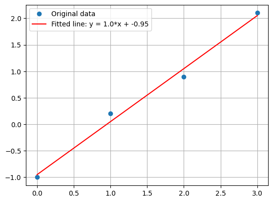
Bonus: Plotting with Python
One nice thing that Numbers gave us was a plot of the data and the line. Python can do this, too, using another fantastic library called Matplotlib. It has good integration with NumPy, and can use the x and y arrays directly. This code (which is also in the notebook):
import matplotlib.pyplot as plt

plt.plot(x, y, "o", label="Original data")
plt.plot(x, m*x + b, "red",
         label=f"Fitted line: y = {m:.2}*x + {b:.2}")
plt.grid(True)
plt.legend()
plt.show()
Produces this plot: